BNMC Blog
Tip of the Week: Handy Excel Functions You May Not Have Known About
There are a lot of functions and capabilities buried in Microsoft Excel, many of which are unknown by most users. This is a real shame, as the value of Excel as a business tool is considerably larger than the simple organization that many see as its limits. To help counteract this, let’s go over a few useful utilities that Excel enables, if you know how to access them.
Count Specific Cells
If you need to take a tally of the number of times a value appears in your spreadsheet, doing so is simple. Using Excel’s COUNTIF function enables you to automatically total up all cells in a given range that meet a given criteria.
Once all your data is entered into a column of your spreadsheet, select a new cell and label it with the data you want to track. In the cell below it, enter the formula =COUNTIF(, then select the range you want to count within (in our case, whichever column contains your data). Once that’s added to your formula, add a comma, and then specify which value you want to tally up in quotes (or, if you’ve labelled another cell with the value, simply select the appropriate cell. Close the parenthesis on your formula, hit enter, and you’re all set.
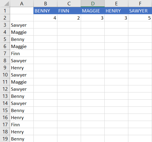
In our example, we get a count of four for “Maggie” by using the formula =COUNTIF(A:A,D1). Alternatively, =COUNTIF(A:A,”Maggie”) would work, too.
Switch Value Format
Here’s the thing: there are a lot of formats that are a pain to type out individually, especially if your raw data isn’t converted. Fortunately, Excel makes it a lot simpler than typing each value out in the correct format. Rather than going through the motions to adjust to the proper formatting for each one, it can be done en masse with just a few clicks. For instance, to change your values to currency, all you must do is highlight the cells you need to change and press Ctrl+Shift+$.
This allows you to turn this:
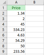
…into this:
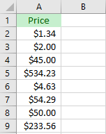
You also have the option to change it using the toolbar. Under Home, you should see a section labelled Number. From there, you have a few quick options to adjust the formatting, including into a few different currencies, as well as a drop-down box with plenty of other options available.

Nicer Formatting
Let’s go back to some basics for a moment with some basic formatting best practices. Without proper formatting, a spreadsheet can be a pain to glean any decent information from, but with the right rules in place, it can quickly gain exponentially more use. Let’s go through a few simple basics to help make your spreadsheets more comprehensible.
Let’s say, for the sake of our example, you wanted to take stock of some of the items in your office. Simple enough—you’d probably begin your list with the title (“Supplies”) and then list what it was you were trying to organize.
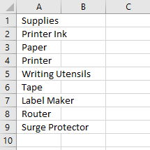
However, with your items varying in length, the spreadsheet could quickly become confusing. Fortunately, this can be fixed by selecting the column and pressing Alt+H+O+I.
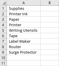
Don’t worry too much if you realize you missed an item… you can always add another row by pressing Ctrl+Shift+Plus Sign.
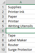
Now that you’ve compiled your list, you don’t want the title “Supplies” to interfere with your amounts. To avoid that, you can merge two cells (in this case, A1 and B1) into a single cell, where “Supplies” will be written out. Select them both and press Alt+H+M+M. Feel free to align your text to the center, as well, by pressing Alt+H+A+C, or by using the icon in the menu bar.
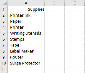
Fill in the number of items you need in the next column over, and the price for each in the column after that (don’t forget to use tip two to change your prices to currency format).
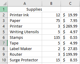
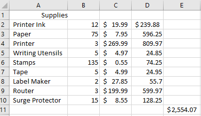
Then, all you need to do is tell Excel to multiply the values in your number of items needed column with the values in your price column, and you’ll have the total needed for each item.
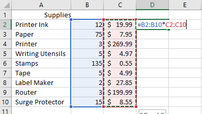
For extra credit, you can then easily add up these costs. Select a new cell, and then click on AutoSum in the Home menu bar. Then, select your final costs, press Enter, and you’ll have the total investment that your supplies will require.
Hopefully, these Excel shortcuts will come in handy. What are some of your favorites? Leave some shortcuts for us to try in the comments!


Comments